Save Time and Avoid Errors in Your Google Sheets Calendars
Do you use Google Sheets to track your to-do lists or do you sell spreadsheets on Etsy? If so, a monthly calendar is a perfect addition to your spreadsheet, as it helps people plan and manage their time.
However, manually entering each month's day is time-consuming and can lead to data entry errors. It's better to have Google Sheets automatically enter the calendar days for you. In this post, I'll show you how!
How to Create Your Automated Calendar
Step #1: Set Up the Calendar Framework
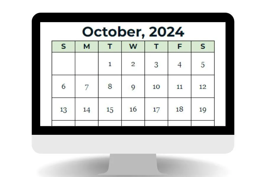
Design your calendar so that it includes:
A cell for the user to select the month and year.
A row that includes the days of the week.
A grid for the dates.
This is how mine looks:

Step #2: Add the Formula to Calculate the First Date of the Month
In the first "day" spot in your calendar grid, I'm using this formula:
=IF(B5="M", $B$4-WEEKDAY($B$4)+2, IF(B5="S", $B$4-WEEKDAY($B$4)+1, ""))
Important: After you copy/paste the formula into your spreadsheet, be sure to replace the cell addresses (B4 and B5) with the correct cell addresses in your spreadsheet.
Formula Cells:
These are my formula cells. However, be sure to change the formula to match your spreadsheet cells!
Cell B4: This is where the user enters the month and year.
Cell B5: The first day of the week; Make sure the “M” and “S” in the formula match the text that’s entered in your calendar. For example, if yours has “Mon,” then change the “M” in the formula to “Mon.” Likewise, make sure that the Sunday text is correct too!
Cell B6: This is where I'm entering this formula.

Step #3: Fill Out the Rest of the Month
Starting with the second day in the grid, enter the formula that adds 1 to the previous day. For example, the formula for the first Monday in cell C6 is B6+1.
In the image below, I made the rows wider so you can see the formulas!

After I entered my formulas, here's how the calendar looks:

Step #4: Remove the Dates from the "Outside" Months
As you can see, the above calendar shows dates for three months:
September 29 and Sept 30
October 1 to 31
November 1 to 9
Since I don't want the September and November dates showing, I'm going to make them invisible:

One way to make the outside days invisible is by applying conditional formatting to the calendar days.
Here's how:
Select Format -> Conditional formatting from the menu bar.
Select your calendar days and apply this rule with the custom formula of:
=MONTH(B6) <> MONTH($B$4)

In the Formatting Style section, make the text color the same color as your date cells. In my spreadsheet, I made the text white.
Here's how my conditional format rule works:
Google Sheets checks each date in the calendar
If the date falls outside of the calendar month that the user entered, then the calendar day color turns to white
If it falls inside the month, then the text color remains black
Grab Your Free Calendar
I hope this tutorial helps you quickly create calendars in Google Sheets.
If you want a copy of the calendar to use as a template, then here you go!
This calendar is currently free with no email address required. I may change that later, but for now, I just want to get this post published!

